Recommendation Systemを考える その2で、機械学習を実施した結果、ロジスティック回帰が良いスコアになったが、その他の分類器ではどうか大まかに調べてみる。
1.複数のアルゴリズムを比較する
ライブラリをインポートする。
# data analysis and wrangling
import pandas as pd
import numpy as np
import random as rnd

# visualization
import matplotlib.pyplot as plt
%matplotlib inline

import seaborn as sns
color = sns.color_palette()
sns.set_style('darkgrid')

import warnings
def ignore_warn(*args, **kwargs):
  pass
warnings.warn = ignore_warn # Ignore annoying warning (from sklearn and seaborn)

# machine learning
from sklearn.linear_model import LogisticRegression
from sklearn.svm import SVC, LinearSVC
from sklearn.ensemble import RandomForestClassifier, AdaBoostClassifier, GradientBoostingClassifier, ExtraTreesClassifier, VotingClassifier
from sklearn.neighbors import KNeighborsClassifier
from sklearn.naive_bayes import GaussianNB
from sklearn.linear_model import Perceptron, SGDClassifier
from sklearn.tree import DecisionTreeClassifier

from sklearn.model_selection import GridSearchCV, cross_val_score, StratifiedKFold, learning_curve
保存しておいたデータを読み込む。
from pathlib import Path

TRAIN_DATA_PATH = str(Path.home()) + '/vscode/syosetu/train_data.pkl'

train = pd.read_pickle(TRAIN_DATA_PATH)
トレーニングデータとテストデータに分割する。
from sklearn.model_selection import train_test_split

X = train['vectors']
y = train['female']

X_array = np.array([np.array(v) for v in X])
y_array = np.array([i for i in y])

X_train, X_test, y_train, y_test = train_test_split(X_array, y_array, random_state=0)
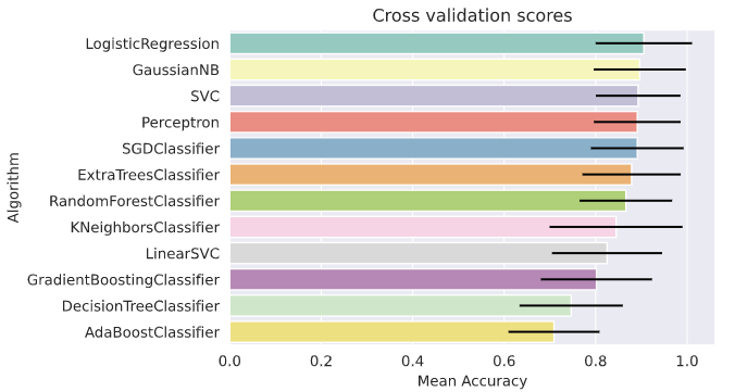
クロスバリデーションのスコアが良い順に表示する。
kfold = StratifiedKFold(n_splits=10)
cls_weight = (y_train.shape[0] - np.sum(y_train)) / np.sum(y_train)
random_state = 0
classifiers = []
classifiers.append(LogisticRegression(random_state=random_state))
classifiers.append(SVC(random_state=random_state))
classifiers.append(KNeighborsClassifier(n_neighbors=3))
classifiers.append(GaussianNB())
classifiers.append(Perceptron(random_state=random_state))
classifiers.append(LinearSVC(random_state=random_state))
classifiers.append(SGDClassifier(random_state=random_state))
classifiers.append(DecisionTreeClassifier(random_state=random_state))
classifiers.append(RandomForestClassifier(n_estimators=100, random_state=random_state))
classifiers.append(AdaBoostClassifier(DecisionTreeClassifier(random_state=random_state), random_state=random_state, learning_rate=0.1))
classifiers.append(GradientBoostingClassifier(random_state=random_state))
classifiers.append(ExtraTreesClassifier(random_state=random_state))

cv_results = []
for classifier in classifiers :
  cv_results.append(cross_val_score(classifier, X_train, y=y_train, scoring='accuracy', cv=kfold, n_jobs=4))

cv_means = []
cv_std = []
for cv_result in cv_results:
  cv_means.append(cv_result.mean())
  cv_std.append(cv_result.std())

cv_res = pd.DataFrame({'CrossVal Means': cv_means, 'CrossVal Errors': cv_std,
                       'Algorithm': ['LogisticRegression', 'SVC', 'KNeighborsClassifier',
                                     'GaussianNB', 'Perceptron', 'LinearSVC', 'SGDClassifier',
                                     'DecisionTreeClassifier', 'RandomForestClassifier',
                                     'AdaBoostClassifier', 'GradientBoostingClassifier',
                                     'ExtraTreesClassifier']})

cv_res.sort_values(by=['CrossVal Means'], ascending=False, inplace=True)

cv_res
| CrossVal Means | CrossVal Errors | Algorithm | |
|---|---|---|---|
| 0 | 0.905357 | 0.105357 | LogisticRegression |
| 3 | 0.896429 | 0.094761 | GaussianNB |
| 1 | 0.892857 | 0.100699 | SVC |
| 4 | 0.891071 | 0.101157 | Perceptron |
| 6 | 0.891071 | 0.101157 | SGDClassifier |
| 11 | 0.878571 | 0.099360 | ExtraTreesClassifier |
| 8 | 0.866071 | 0.120387 | RandomForestClassifier |
| 2 | 0.844643 | 0.092461 | KNeighborsClassifier |
| 5 | 0.825000 | 0.107381 | LinearSVC |
| 10 | 0.801786 | 0.112783 | GradientBoostingClassifier |
| 7 | 0.746429 | 0.145248 | DecisionTreeClassifier |
| 9 | 0.708929 | 0.121389 | AdaBoostClassifier |
回帰系のアルゴリズムでスコアが良い傾向があるように見える。
g = sns.barplot('CrossVal Means', 'Algorithm', data=cv_res, palette='Set3', orient='h', **{'xerr': cv_std})
g.set_xlabel('Mean Accuracy')
g = g.set_title('Cross validation scores')
2.パラメーターの最適化
続いて、いくつか選んだアルゴリズムのパラメーターを変更して、スコアの変化を見てみる。
### META MODELING WITH LR, RF and SGD

# Logistic Regression
LR = LogisticRegression(random_state=0)

## Search grid for optimal parameters
lr_param_grid = {'penalty': ['l1','l2']}

gsLR = GridSearchCV(LR, param_grid=lr_param_grid, cv=kfold, scoring='accuracy', n_jobs=4, verbose=1)

gsLR.fit(X_train, y_train)

LR_best = gsLR.best_estimator_

# Best score
gsLR.best_score_
Fitting 10 folds for each of 2 candidates, totalling 20 fits
0.9053571428571429
gsLR.best_params_
{‘penalty’: ‘l2’}
# Random Forest Classifier
RF = RandomForestClassifier(random_state=0)

## Search grid for optimal parameters
'''rf_param_grid = {'criterion': ['gini', 'entropy'],
                 'max_features': [1, 3, 10],
                 'min_samples_split': [2, 3, 10],
                 'min_samples_leaf': [1, 3, 10],
                 'n_estimators':[50, 100, 200]}'''
rf_param_grid = {'criterion': ['gini', 'entropy'],
                 'max_features': [40, 50, 60],
                 'min_samples_split': [2, 3, 10],
                 'min_samples_leaf': [1, 3, 10],
                 'n_estimators':[20, 30, 40]}

gsRF = GridSearchCV(RF, param_grid=rf_param_grid, cv=kfold, scoring='accuracy', n_jobs=4, verbose=1)

gsRF.fit(X_train, y_train)

RF_best = gsRF.best_estimator_

# Best score
gsRF.best_score_
Fitting 10 folds for each of 162 candidates, totalling 1620 fits
0.8946428571428573
gsRF.best_params_
{‘criterion’: ‘gini’,
‘max_features’: 50,
‘min_samples_leaf’: 3,
‘min_samples_split’: 2,
‘n_estimators’: 30}
# SGD Classifier
SGD = SGDClassifier(random_state=0)

## Search grid for optimal parameters
sgd_param_grid = {'alpha'  : [0.0001, 0.001, 0.01, 0.1],
                  'loss'   : ['log', 'modified_huber'],
                  'penalty': ['l2', 'l1', 'none']}

gsSGD = GridSearchCV(SGD, param_grid=sgd_param_grid, cv=kfold, scoring='accuracy', n_jobs=4, verbose=1)

gsSGD.fit(X_train, y_train)

SGD_best = gsSGD.best_estimator_

# Best score
gsSGD.best_score_
Fitting 10 folds for each of 24 candidates, totalling 240 fits
0.8660714285714285
gsSGD.best_params_
{‘alpha’: 0.0001, ‘loss’: ‘modified_huber’, ‘penalty’: ‘l1’}
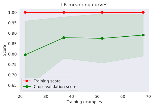
3.学習曲線の確認
def plot_learning_curve(estimator, title, X, y, ylim=None, cv=None,
n_jobs=-1, train_sizes=np.linspace(.1, 1.0, 5)):
'''Generate a simple plot of the test and training learning curve'''
plt.figure()
plt.title(title)
if ylim is not None:
plt.ylim(*ylim)
plt.xlabel('Training examples')
plt.ylabel('Score')
train_sizes, train_scores, test_scores = learning_curve(
estimator, X, y, cv=cv, n_jobs=n_jobs, train_sizes=train_sizes)
train_scores_mean = np.mean(train_scores, axis=1)
train_scores_std = np.std(train_scores, axis=1)
test_scores_mean = np.mean(test_scores, axis=1)
test_scores_std = np.std(test_scores, axis=1)
plt.grid()
plt.fill_between(train_sizes, train_scores_mean - train_scores_std,
train_scores_mean + train_scores_std, alpha=0.1,
color='r')
plt.fill_between(train_sizes, test_scores_mean - test_scores_std,
test_scores_mean + test_scores_std, alpha=0.1,
color='g')
plt.plot(train_sizes, train_scores_mean, 'o-', color='r',
label='Training score')
plt.plot(train_sizes, test_scores_mean, 'o-', color='g',
label='Cross-validation score')
plt.legend(loc='best')
return plt
g = plot_learning_curve(gsLR.best_estimator_, 'LR mearning curves', X_train, y_train, cv=kfold)
g = plot_learning_curve(gsRF.best_estimator_, 'RF learning curves', X_train, y_train, cv=kfold)
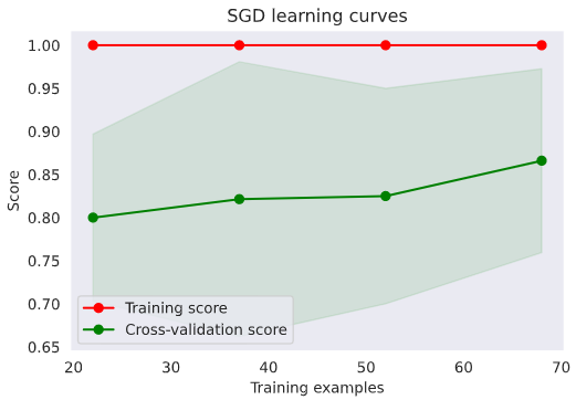
g = plot_learning_curve(gsSGD.best_estimator_, 'SGD learning curves', X_train, y_train, cv=kfold)
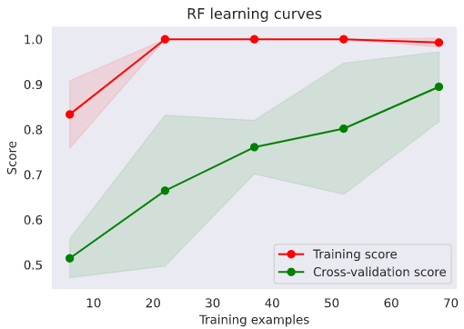
Random Forestも良い気がしてきた。何とかトレーニングデータを増やしてもう少し確認したい。
最後に
全くトレーニングで使用していない未知のデータに対して、 Random Forest の予測モデルで判定してみたところ83%程の正解率だった。なろう小説のTop300はファンタジー系の小説が多いため、ファンタジー系の小説において、この正解率とみた方が良いかも知れない。ジャンルが違う小説の場合どのような結果になるか現時点では予測不能である。